LSTM Forward and Backward Pass

Introduction

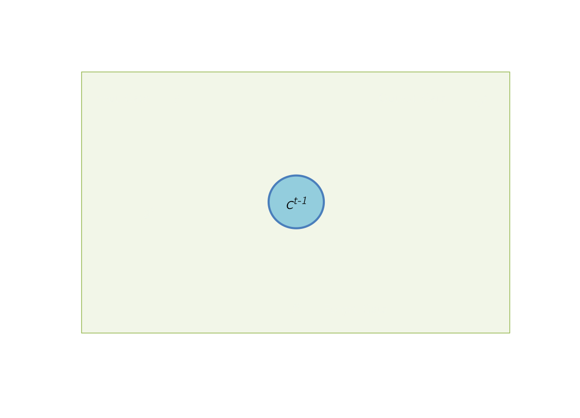
Forward Pass: Initial State

Initially, at time \(t\), the memory cells of the LSTM contain values from the previous iteration at time \( (t-1) \).

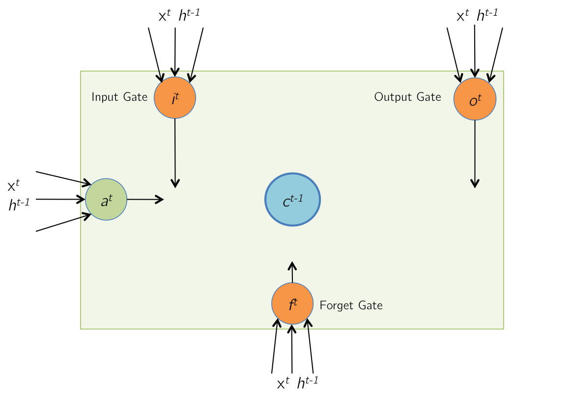
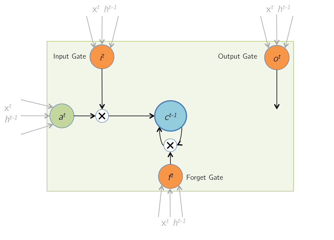
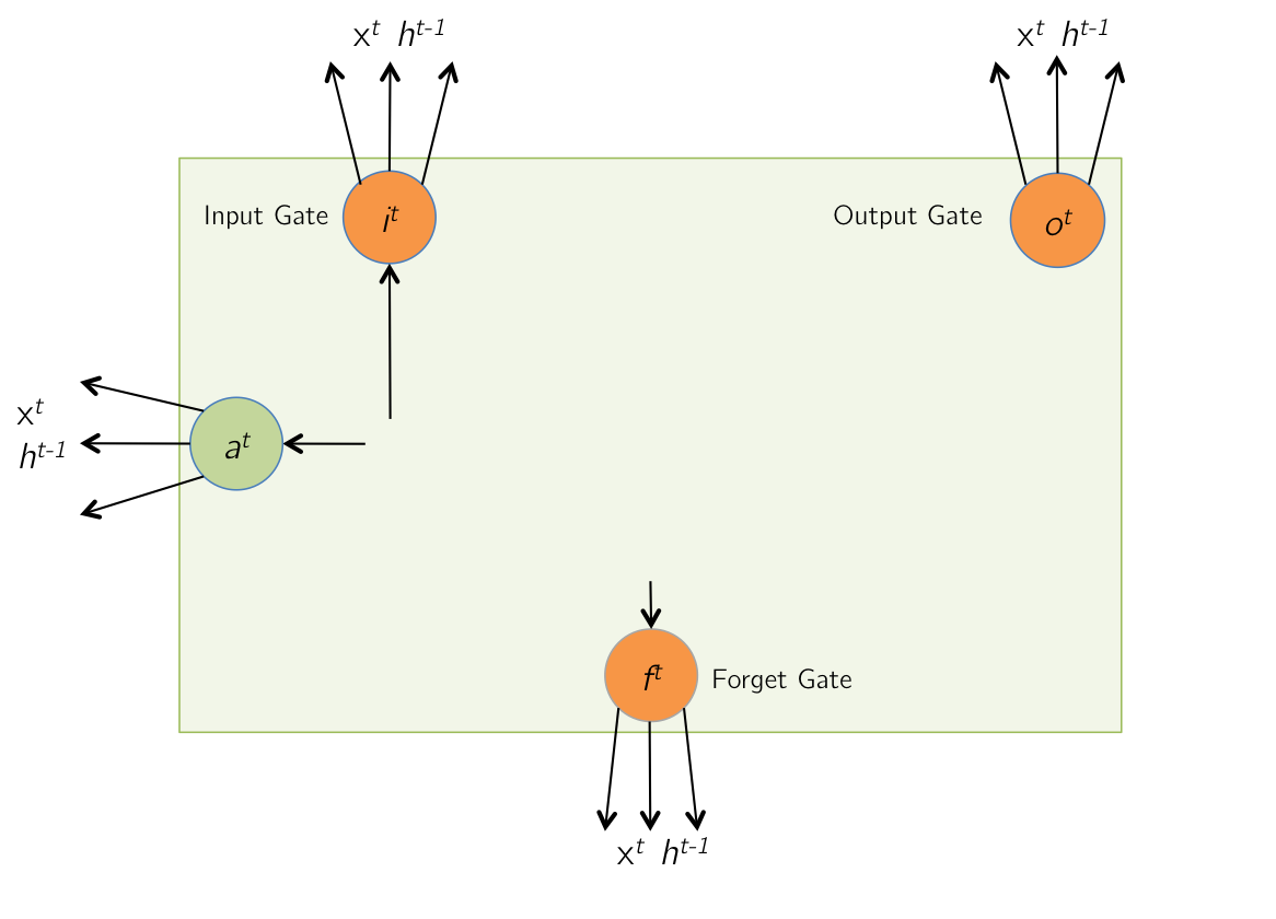
Forward Pass: Input and Gate Computation

At time \( t \), The LSTM receives a new input vector \( x^t \) (including the bias term), as well as a vector of its output at the previous timestep, \( h^{t-1} \).

\begin{align} a^t &= \tanh(W_cx^t + U_ch^{t-1}) = \tanh(\hat{a}^t) \\ i^t &= \sigma(W_ix^t + U_ih^{t-1}) = \sigma(\hat{i}^t) \\ f^t &= \sigma(W_fx^t + U_fh^{t-1}) = \sigma(\hat{f}^t) \\ o^t &= \sigma(W_ox^t + U_oh^{t-1}) = \sigma(\hat{o}^t) \end{align} Ignoring the non-linearities, \begin{align} z^t = \begin{bmatrix} \hat{a}^t \\ \hat{i}^t \\ \hat{f}^t \\ \hat{o}^t \end{bmatrix} &= \begin{bmatrix} W^c & U^c \\ W^i & U^i \\ W^f & U^f \\ W^o & U^o \end{bmatrix} \times \begin{bmatrix} x^t \\ h^{t-1} \end{bmatrix} \\ &= W \times I^t \end{align}

If the input \(x^t\) is of size \(n \times 1\), and we have \(d\) memory cells, then the size of each of \(W_\ast\) and \(U_\ast\) is \(d \times n\), and and \(d \times d \) resp. The size of \(W\) will then be \(4d \times (n+d)\). Note that each one of the \(d\) memory cells has its own weights \(W_\ast\) and \(U_\ast\), and that the only time memory cell values are shared with other LSTM units is during the product with \(U_\ast\).

Forward Pass: Memory Cell Update

During this step, the values of the memory cells are updated with a combination of \( a^t \), and the previous cell contents \( c^{t-1} \). The combination is based on the magnitudes of the input gate \( i^t \) and the forget gate \( f^t \). \( \odot \) denotes elementwise product (Hadamard product).

$$ c^t = i^t \odot a^t + f^t \odot c^{t-1} $$

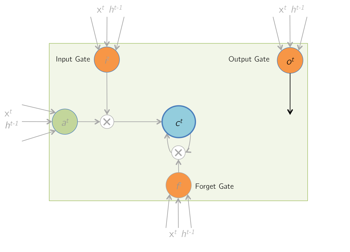
Forward Pass: Updated Memory Cells

The contents of the memory cells are updated to the latest values.

$$ c^{t-1} \rightarrow c^t $$

Forward Pass: Output

Finally, the LSTM cell computes an output value by passing the updated (and current) cell value through a non-linearity. The output gate determines how much of this computed output is actually passed out of the cell as the final output \( h^t \).

$$ h^t = o^t \odot \text{tanh}(c^t) $$

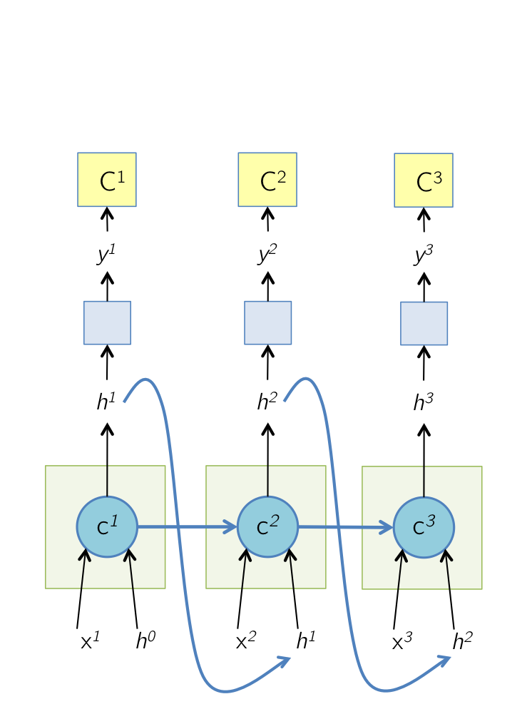
Forward Pass: Unrolled Network

The unrolled network during the forward pass is shown below. Note that the gates have not been shown for brevity. An interesting point to note here is that in the computational graph below, the cell state at time \( T \), \( c^T \) is responsible for computing \( h^T \) as well as the next cell state \( c^{T+1} \). At each time step, the cell output \( h^T \) is shown to be passed to some more layers on which a cost function \( C^T \) is computed, as the way an LSTM would be used in a typical application like captioning or language modeling.

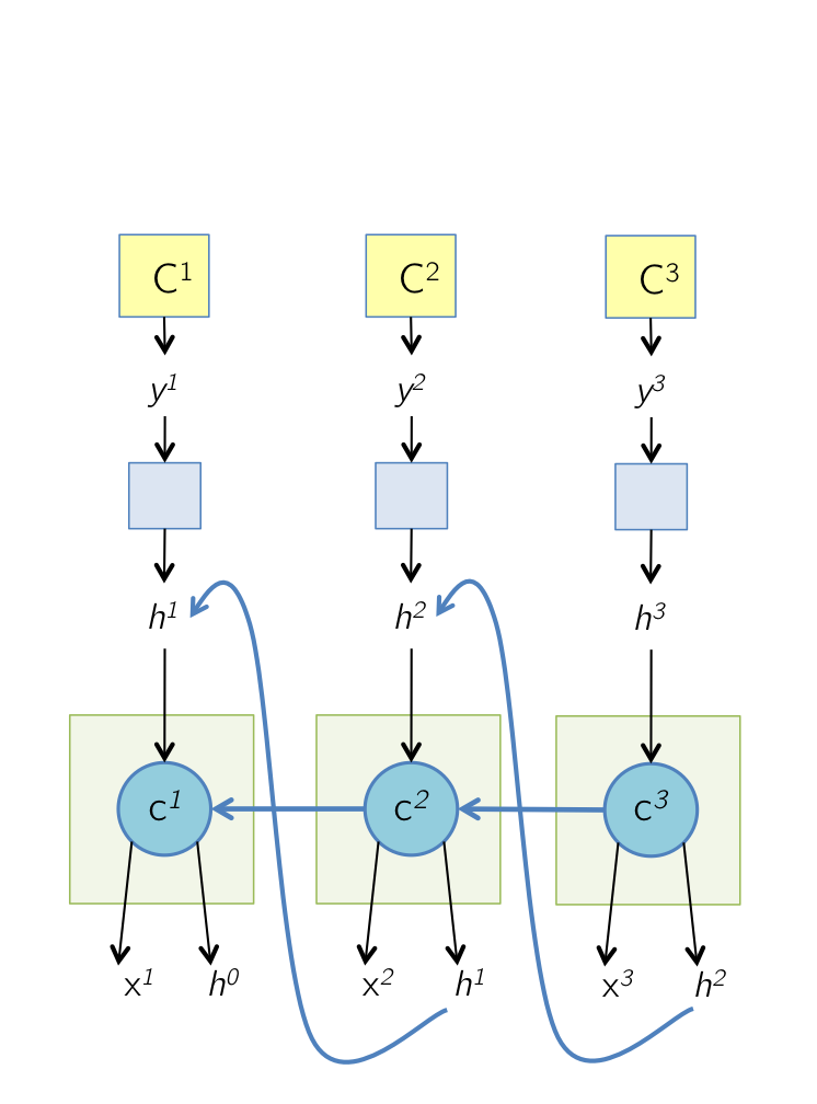
Backward Pass: Unrolled Network

The unrolled network during the backward pass is shown below. All the arrows in the previous slide have now changed their direction. The cell state at time \( T \), \( c^T \) receives gradients from \( h^T \) as well as the next cell state \( c^{T+1} \). The next few slides focus on computing these two gradients. At any time step \( T \), these two gradients are accumulated before being backpropagated to the layers below the cell and the previous time steps.

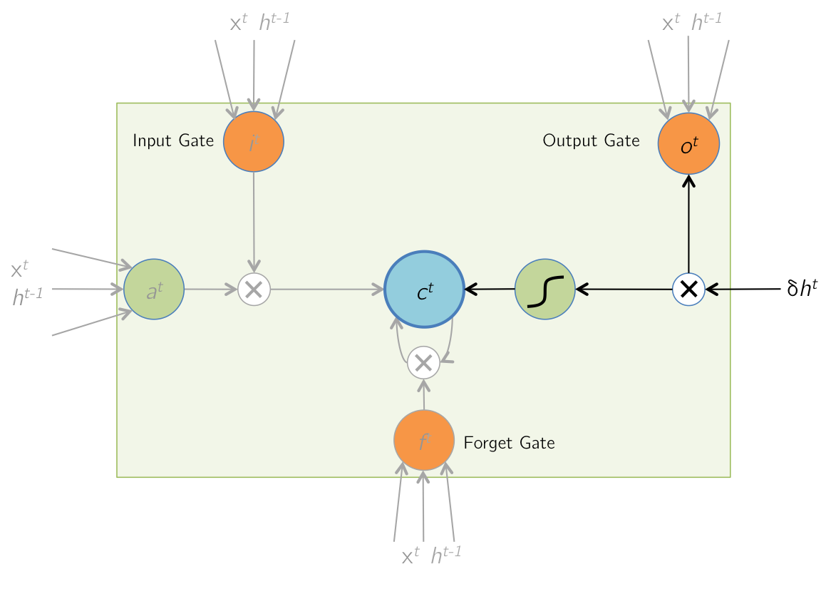
Backward Pass: Output

\begin{align} \text{Forward Pass: } h^t &= o^t \odot \tanh(c^t) \\ \text{Given } \delta h^t &= \displaystyle\frac{\partial E}{ \partial h^t}, \text{find } \delta o^t, \delta c^t \end{align} \begin{align} \frac{\partial E}{\partial o^t_i} &= \frac{\partial E}{\partial h^t_i} \cdot \frac{\partial h^t_i}{\partial o^t_i}\\ &= \delta h^t_i \cdot \tanh(c^t_i) \\ \therefore \delta o^t &= \delta h^t \odot \tanh(c^t)\\ \\ \frac{\partial E}{\partial c^t_i} &= \frac{\partial E}{\partial h^t_i} \cdot \frac{\partial h^t_i}{\partial c^t_i}\\ &= \delta h^t_i \cdot o^t_i \cdot (1-\tanh^2(c^t_i))\\ \therefore \delta c^t & \color{red}+= \color{black}\delta h^t \odot o^t \odot (1-\tanh^2(c^t)) \end{align} Note that the \(\color{red} += \) above is so that this gradient is added to gradient from time step \( (t+1) \) (calculated on next slide, refer to the gradient accumulation mentioned in the previous slide)

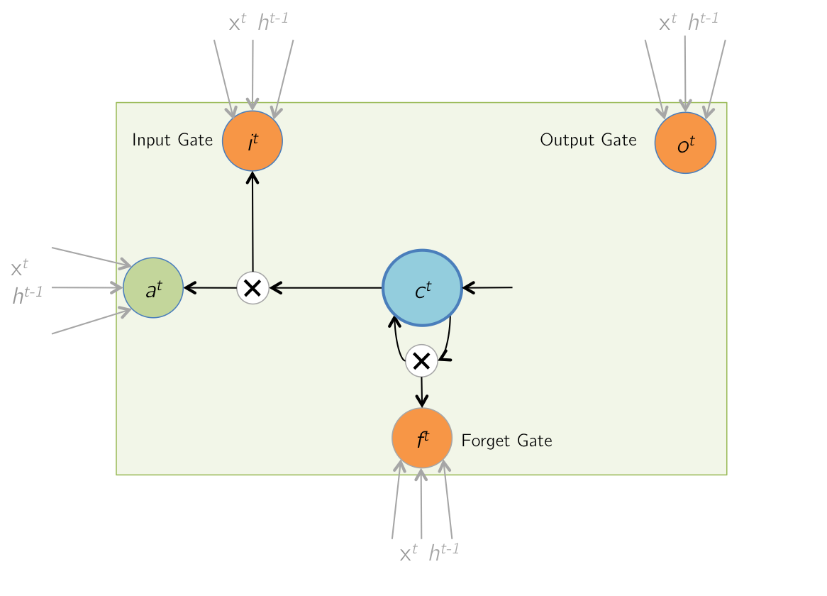
Backward Pass: LSTM Memory Cell Update

\begin{align} \text{Forward Pass: } c^t &= i^t \odot a^t + f^t \odot c^{t-1} \\ \text{Given } \delta c^t &= \displaystyle\frac{\partial E}{ \partial c^t}, \text{find } \delta i^t, \delta a^t, \delta f^t, \delta c^{t-1} \end{align} \begin{array}{l|l} \begin{align} \frac{\partial E}{\partial i^t_i} &= \frac{\partial E}{\partial c^t_i} \cdot \frac{\partial c^t_i}{\partial i^t_i} & \frac{\partial E}{\partial f^t_i} &= \frac{\partial E}{\partial c^t_i} \cdot \frac{\partial c^t_i}{\partial f^t_i}\\ &= \delta c^t_i \cdot a^t_i & &= \delta c^t_i \cdot c^{t-1}_i\\ \therefore \delta i^t &= \delta c^t \odot a^t & \therefore \delta f^t &= \delta c^t \odot c^{t-1}\\ \\ \frac{\partial E}{\partial a^t_i} &= \frac{\partial E}{\partial c^t_i} \cdot \frac{\partial c^t_i}{\partial a^t_i} & \frac{\partial E}{\partial c^{t-1}_i} &= \frac{\partial E}{\partial c^t_i} \cdot \frac{\partial c^t_i}{\partial c^{t-1}_i}\\ &= \delta c^t_i \cdot i^t_i & &= \delta c^t_i \cdot f^t_i \\ \therefore \delta a^t &= \delta c^t \odot i^t & \therefore \delta c^{t-1} &= \delta c^t \odot f^t \end{align} \end{array}

Backward Pass: Input and Gate Computation - I

\begin{align} \text{Forward Pass: } z^t &= \begin{bmatrix} \hat{a}^t \\ \hat{i}^t \\ \hat{f}^t \\ \hat{o}^t \end{bmatrix} = W \times I^t \\ \text{Given } \delta a^t, \delta i^t , &\delta f^t, \delta o^t, \text{ find } \delta z^t \end{align} \begin{array}{l|l} \begin{align} \delta \hat{a}^t &= \delta a^t \odot (1-\tanh^2(\hat{a}^t)) \\ \delta \hat{i}^t &= \delta i^t \odot i^t \odot (1-i^t) \\ \delta \hat{f}^t &= \delta f^t \odot f^t \odot (1-f^t) \\ \delta \hat{o}^t &= \delta o^t \odot o^t \odot (1-o^t) \\ \delta z^t &= \left[ \delta\hat{a}^t, \delta\hat{i}^t, \delta\hat{f}^t, \delta\hat{o}^t \right]^T \end{align} \end{array}

Backward Pass: Input and Gate Computation - II

\begin{align} \text{Forward Pass: } z^t &= W \times I^t \\ \text{Given } \delta z^t, \text{ find }& \delta W^t, \delta h^{t-1} \end{align} \begin{align} \delta I^t &= W^T \times \delta z^t\\ \text{As } I^t &= \begin{bmatrix} x^t \\ h^{t-1} \end{bmatrix} \text{, }\\ \delta h^{t-1} &\text{ can be retrieved from } \delta I^t\\ \delta W^t &= \delta z^t \times (I^t)^T\\ \end{align}

Parameter Update