A Quick Introduction to Backpropagation
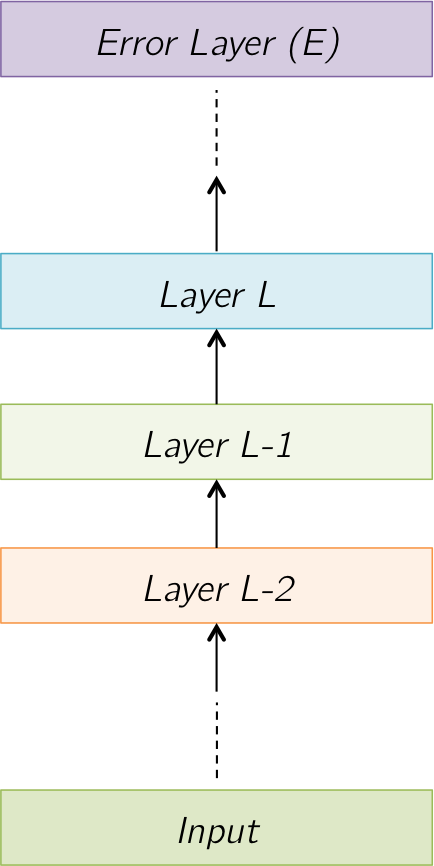
Consider a network made of multiple layers, connected to some error function \( E(\cdot) \) at the top, as shown in the figure below. Each layer takes in some input, transforms it in some fashion, and then produces some output, which is then passed on to the next layer, until the error layer is reached. Once the error is computed with respect to the target, corrective gradients are passed down to change the network parameters.
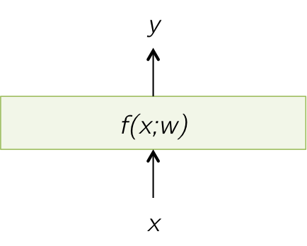
Most layers can be represented as applying some function \(f(\cdot)\) with parameters \(w\), on the input vector \(x\) of length \(m\) to produce output \(y\) of length \(n\). We'll use \(i\) to index values of \(x\) and \(j\) to index values of \(y\) in the parts that follow. Some layers might take in or produce multiple input/output values. A simple example is a loss layer which takes in input predictions and truth targets and then produces a corresponding error value. Some layers might not have any parameters \(w\) but instead just apply a fixed function. Examples of such layers include loss layers and non-linearity layers such as sigmoid, tanh, ReLU.
In the parts that follow, we'll look at some common layers and derive backpropagation equations for them.
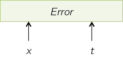
The Euclidean Loss Layer takes in some input \(x\) and measures how far this input is from the expected targets \(t\) using the equation below. This layer technically produces the amount of error as its output, but loss layers are the end of a network, and its output is not passed on to any layer. So, our \(y\) here is non-existent. Also, this error (loss) function is not parameterized by any weights \(w\) as shown below.
Error \( = E = \displaystyle\frac{1}{2}\displaystyle\sum_{i=1}^m (x_i - t_i)^2 \)
\begin{align} \frac{\partial E}{\partial x_i} &= \frac{1}{2} \cdot 2 \cdot (x_i - t_i) = (x_i - t_i)\\ \delta x &= \left[ \frac{\partial E}{\partial x_i} \right]_i = x - t \end{align} \(\delta x\) and \( t \) are of size \(m \times 1\) $$ \boxed{ \begin{align} \delta x &= x - t \\ \delta w &= \text{N.A.} \end{align} } $$
The log loss also measure the deviation of the input \(x\) from the true output targets \(t\), but using a different equation shown below.
Error \( = E = -\displaystyle\sum_{i=1}^m t_i \log x_i \)
\begin{align} \frac{\partial E}{\partial x_i} &= -\frac{t_i}{x_i} \\ \delta x &= \left[ \frac{\partial E}{\partial x_i} \right]_i = - t \odot \frac{1}{x} \end{align} \(\delta x\) and \( t \) are of size \(m \times 1\) $$ \boxed{ \begin{align} \delta x &= - t \odot \frac{1}{x} \\ \delta w &= \text{N.A.} \end{align} } $$
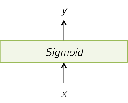
The sigmoid layer takes in some input \(x\) and applies the sigmoid function on each value in \(x\) to produce output \(y\). The sigmoid function too, does not have any parameters \(w\). It just applies a fixed transformation shown below, on each input value. $$ y_i = \frac{1}{1+e^{-x_i}} $$
\begin{align} \frac{\partial E}{\partial x_i} &= \frac{\partial E}{\partial y_i} \cdot \frac{\partial y_i}{\partial x_i} = \delta y_i \cdot \frac{\partial y_i}{\partial x_i}\\ \frac{\partial y_i}{\partial x_i} &= \frac{e^{-x_i}}{(1+e^{-x_i})^2} = y_i \cdot (1-y_i)\\ \therefore \frac{\partial E}{\partial x_i} &= \delta y_i \cdot y_i \cdot (1-y_i)\\ \delta x &= \left[ \frac{\partial E}{\partial x_i} \right]_i = \delta y \odot y \odot (1-y) \end{align} Note that in this layer, \( m=n \) \(\delta x\) is of size \(m \times 1\), \(\delta y\) is of size \(n \times 1\), \(y\) and \((1-y)\) are of size \(n \times 1\) $$ \boxed{ \begin{align} \delta x &= \delta y \odot y \odot (1-y) \\ \delta w &= \text{N.A.} \end{align} } $$
The softmax layer normalizes its inputs \(x\) to produce outputs \(y\) such that sum of output values is 1, using the equation below. This layer is used to produce outputs which can be interpreted as probability distributions. It is thus very commonly used in networks predicting class probabilities of inputs. Note that an output \(y_j\) depends on every input \(x_i\). $$ y_i = \frac{e^{x_i}}{\sum_{k=1}^m e^{x_k}} $$
\begin{align} \frac{\partial E}{\partial x_i} &= \sum_{j=1}^n \left( \frac{\partial E}{\partial y_j} \cdot \frac{\partial y_j}{\partial x_i} \right)\\ \text{If } i=j, \frac{\partial y_i}{\partial x_i} &= \frac{\partial}{\partial x_i} \left\{ \frac{e^{x_i}}{\sum_{k=1}^m e^{x_k}} \right\}\\ &= \frac{ e^{x_i}\left(\sum_{k=1}^m e^{x_k}\right) - \left(e^{x_i}\right)^2} { \left(\sum_{k=1}^m e^{x_k}\right)^{2} } \\ &= \frac{ e^{x_i} } { \sum_{k=1}^m e^{x_k} }- \frac{ \left(e^{x_i}\right)^2 } { \left(\sum_{k=1}^m e^{x_k}\right)^{2} } \\ &= \frac{ e^{x_i} } { \sum_{k=1}^m e^{x_k} } \left( 1- \frac{ e^{x_i} } { \sum_{k=1}^m e^{x_k} } \right) \\ &= y_i \cdot (1-y_i)\\ &= y_i \cdot (\mathbf{1}\{ i=j \} - y_j)\\ \text{If } i\neq j, \frac{\partial y_i}{\partial x_i} &= \frac{\partial}{\partial x_i} \left\{ \frac{e^{x_j}}{\sum_{k=1}^m e^{x_k}} \right\}\\ &= \frac{-e^{x_i}\cdot e^{x_j}}{\left(\sum_{k=1}^m e^{x_k}\right)^2} \\ &= \frac{-e^{x_i}}{\sum_{k=1}^m e^{x_k}} \cdot \frac{e^{x_j}}{\sum_{k=1}^m e^{x_k}}\\ &= -y_i \cdot y_j\\ &= y_i \cdot (\mathbf{1}\{ i=j \} - y_j) \end{align}
\begin{align} \therefore \frac{\partial E}{\partial x_i} &= \sum_{j=1}^n \delta y_j \cdot y_i \cdot (\mathbf{1}\{ i=j \} - y_j)\\ &= \sum_{j=1}^n J_{ij} \times \delta y_j\\ \text{where } J_{ij} &= y_i \cdot (\mathbf{1}\{ i=j \} - y_j)\\ \delta x &= \left[ \frac{\partial E}{\partial x_i} \right]_i = J \times \delta y \end{align}
Note that in this layer, \( m=n \) \(\delta x\) is of size \(m \times 1\), \( J \) is of size \( m \times n \), \(\delta y\) is of size \(n \times 1\)
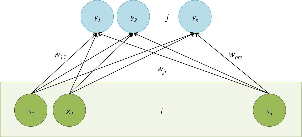
$$ \boxed{ \begin{align} \delta x &= J \times \delta y \\ \delta w &= \text{N.A.} \end{align} } $$In the fully connected layer, each output neuron \(y_1, \cdots, y_n \) is connected to each input value \(x_1, \cdots, x_m\) with a weight \(w_{ji}\). The collection of all weights, \( W = \{ w_{ji} \} \), is the set of parameters of this layer. \(W\) is a matrix of size \( n \times m \). The relationship between the inputs and outputs is shown below.
\( y_j = \displaystyle\sum_{i=1}^m w_{ji} \cdot x_i \) or equivalently in matrix form, \( y = W \times x \), where \(W = \left[ w_{ji} \right]\) is of size \( n \times m \)
 $$
\begin{align}
\frac{\partial E}{\partial x_{i}} &= \sum_{j=1}^n \left( \frac{\partial E}{\partial y_j} \cdot \frac{\partial y_j}{\partial x_i} \right) \\
\frac{\partial y_j}{\partial x_i} &= \frac{\partial \left( \displaystyle\sum_{i=1}^m w_{ji} \cdot x_i\right)}{\partial x_i} = w_{ji}\\
\therefore \frac{\partial E}{\partial x_{i}} &= \sum_{j=1}^n \left( \delta y_j \cdot w_{ji} \right) = \sum_{j=1}^n \left( w^T_{ij} \cdot \delta y_j \right)\\
\delta x &= \left[ \frac{\partial E}{\partial x_{i}} \right]_i = W^T \times \delta y
\end{align}
$$
\(\delta x\) is of size \(m \times 1\), \(W^T\) is of size \(m \times n\), \(y\) is of size \(n \times 1\)
$$
\begin{align}
\frac{\partial E}{\partial x_{i}} &= \sum_{j=1}^n \left( \frac{\partial E}{\partial y_j} \cdot \frac{\partial y_j}{\partial x_i} \right) \\
\frac{\partial y_j}{\partial x_i} &= \frac{\partial \left( \displaystyle\sum_{i=1}^m w_{ji} \cdot x_i\right)}{\partial x_i} = w_{ji}\\
\therefore \frac{\partial E}{\partial x_{i}} &= \sum_{j=1}^n \left( \delta y_j \cdot w_{ji} \right) = \sum_{j=1}^n \left( w^T_{ij} \cdot \delta y_j \right)\\
\delta x &= \left[ \frac{\partial E}{\partial x_{i}} \right]_i = W^T \times \delta y
\end{align}
$$
\(\delta x\) is of size \(m \times 1\), \(W^T\) is of size \(m \times n\), \(y\) is of size \(n \times 1\)
$$ \begin{align} \frac{\partial E}{\partial w_{ji}} &= \frac{\partial E}{\partial y_j} \cdot \frac{\partial y_j}{\partial w_{ji}} = \delta y_j \cdot \frac{\partial y_j}{\partial w_{ji}}\\ \frac{\partial y_j}{\partial w_{ji}} &= \frac{\partial \left( \displaystyle\sum_{i=1}^m w_{ji} \cdot x_i\right)}{\partial w_{ji}} = x_i\\ \therefore \frac{\partial E}{\partial w_{ji}} &= \delta y_j \cdot x_i\\ \delta w &= \left[ \frac{\partial E}{\partial w_{ji}} \right]_{ji} = \delta y \times x^T \\ \end{align} $$
\(\delta w\) is of size \(n \times m\), \(\delta y\) is of size \(n \times 1\), \(x^T\) is of size \(1 \times m\)
$$ \boxed{ \begin{align} \delta x &= W^T \times \delta y \\ \delta w &= \delta y \times x^T \end{align} } $$